Last Updated On: 2020-07-11 16:31

Autoencoders

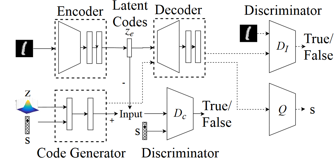
Table of Content

• Autoencoders
  • Table of Content
  • Introduction
  • Vanilla Autoencoder model and its variants
  • Regularized Autoencoders
  • Denoising Autoencoder
  • Sparse Autoencoder
  • Contractive Autoencoder
  • Variational Autoencoder
    • Mathematics
      • Expectation
      • Bayes Theorem
      • Naive Bayes Algorithm and its training strategies
      • Variational Inference
      • Kullback-Leibler (KL) Divergence
    • What VAE Offers
    • VAE Loss function Derivation
      • Derivative of loss function
    • Matrix Maths and Training
  • Conditional Variational Autoencoders
  • Adversarial Autoencoders
    • Tensorflow Implementation
  • References
• Comments

Introduction

• Type of Autoencoders
  • Vanilla Encoder Decoder model and its variants
  • Regularized Autoencoders
  • Sparse Autoencoders
  • Denoising Autoencoders
  • Contractive Autoencoders
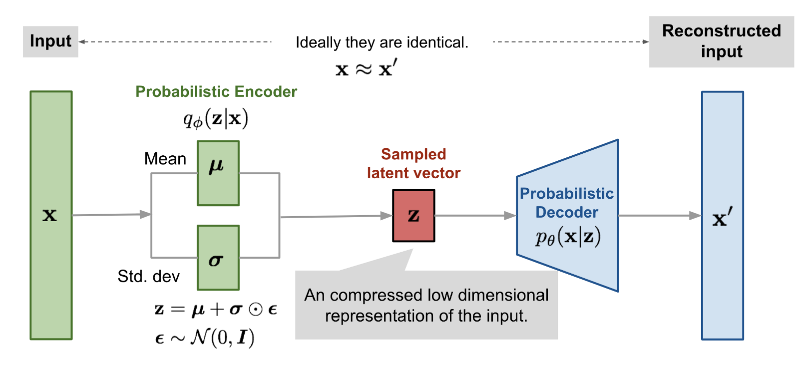
  • Variational Autoencoders
  • Conditional Variational Autoencoders
  • Adversarial Autoencoders

Vanilla Autoencoder model and its variants

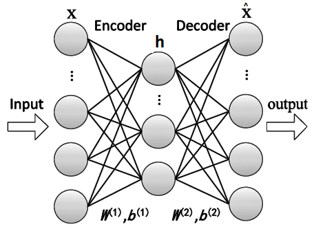
• Simple Encoder Decoder models.

• Condensed vector representation of Input.

• Autoencoder without activation function and mean squared error as loss function is same as PCA(Principal Component Analysis).

• Sometimes the optimal model comes out to be a linear model(PCA), means without activation functions {it can be proved by using singular value decomposition}.

• Undercomplete and overcomplete Autoencoder

  • Undercomplete : Hidden layer (condensed latent vector) has lower dimension then the input.

  • Overcomplete : Hidden layer has higher dimension then the input.

    

• One Layer Encoder

  $\begin{aligned} h & = g(a(X)) \\ & = \sigma(b^{(1)} + W^{(1)}X) \end{aligned}$

• One Layer Decoder
  $\begin{aligned} \hat{X} & = o(\hat{a}(X)) \\ & = \sigma(b^{(2)} + W^{(2)}X) \end{aligned}$

• Loss function and its derivative
  $\begin{aligned} L(\hat{y}, y) &=\frac{1}{n}\sum_{i=1}^{n}(\hat{y_i}-y_i)^2 \tag{1} \\ \nabla{L(\hat{y}, y)} &= \hat{y} - y \end{aligned}$
  $\begin{aligned} L(\hat{y}, y)&=-\sum_{i=1}^{n}(ylog(\hat{y}) + (1-y)log(1-\hat{y})) \tag{2} \\ \nabla{L(\hat{y}, y)} &= \frac{\hat{y} - y}{(1-\hat{y})(y)} \end{aligned}$

  (1) mean squared error, maximum likelihood, sum squared error, or Squared Euclidean Distance
  (2) Bernoulli negative log-likelihood, or Binary Cross-Entropy

• Backpropogation(Weight Updation)

Regularized Autoencoders

• L1 and L2 Regularization
  • L1 Regularization : $L(\hat{y}, y) =\frac{1}{n}\sum_{i=1}^{n}(\hat{y_i}-y_i)^2+\lambda|\theta|$
  • L2 Regularization : $L(\hat{y}, y) =\frac{1}{n}\sum_{i=1}^{n}(\hat{y_i}-y_i)^2+\lambda|\theta|^2$

Denoising Autoencoder

• DAEs take a partially corrupted input and are trained to recover the original undistorted input
• Stocastic mapping procedure is used to corrupt the data

Sparse Autoencoder

• Sparse autoencoder may include more (rather than fewer) hidden units than inputs, but only a small number of the hidden units are allowed to be active at once.

• Loss Function
  $\begin{aligned} L(\hat{y}, y) =\frac{1}{n}\sum_{i=1}^{n}(\hat{y_i}-y_i)^2 + \Omega{(h)}\tag{3} \end{aligned}$

  $\Omega{(h)}$ : sparsity penalty

Contractive Autoencoder

• Loss Function
  $\begin{aligned} L(\hat{y}, y) =\frac{1}{n}\sum_{i=1}^{n}(\hat{y_i}-y_i)^2 + \lambda{\sum||\nabla_y{h_i}||^2}\tag{3} \end{aligned}$

  $\lambda{\sum||\nabla_y{h_i}||^2}$ : Frobenius Norm

Variational Autoencoder

Mathematics

• Expectation Value
• Monte Carlo Estimation of Expectation
• Bayes Theorem
• Naive Bayes Algorithm and its trainig strategies
• Variational Inference
• KL divergence

Expectation

• Expectation or Expected value of some random variable X with outcomes(finite) as $\{x_1,x_2,...,x_k\}$ with probabilities as $\{p_{x_1},p_{x_2},...,p_{x_k}\}$

$E(X) = \sum_i^k{x_ip_{x_i}}$

• X is a continuous event the change summation to integral.

• Conditional Expectation

$E(X|Z) = \frac{\sum_{z \in Z}{X(z)}}{|Z|} \hspace{30pt} \forall \hspace{30pt} Z = \{z_1,z_2,...z_k\}$

• $|Z|$ is called cardinality of Z

Bayes Theorem

• More elaborate guide is here

• In probability theory and statistics, Bayes' theorem (alternatively Bayes's theorem, Bayes's law or Bayes's rule) describes the probability of an event, based on prior knowledge of conditions that might be related to the even [wikipedia defination]

• Bayes theorem gives the measure of the probability of a hypothesis z, given some new data x.

$p(z|x) = \frac{p(x|z)p(z)}{p(x)}$

• Its Derivation
  $\begin{aligned} p(x \cap y) &= p(y \cap x) \\ p(x|y)p(y) &= p(y|x)p(x) \\ p(x|y) &= \frac{p(y|x)p(x)}{p(y)} \end{aligned}$

Naive Bayes Algorithm and its training strategies

Ref : http://www.cs.cornell.edu/courses/cs4780/2018sp/lectures/lecturenote05.html

• Bayesian Classification : Lets assume that $L = \{l_1,l_2,...,l_k\}$ labels has to be predicted using a data point $X=\{x_1,x_2,X_3,...,x_n\}$, hence the probalitistic output(i.e class score) of the event is,

  $P(L|X)$

  And, According to the Bayes Theorem.

  $P(L|X) = \frac{P(X|L)P(L)}{P(X)}$

• So, if we some how calculate the value of $P(X|L)$ then the problem is solved. Such type of probilistic model is called generative modeling in which we are generating data given its label. In general such training is very difficult.

• First naive bayes assumption: feature values$(X)$ are independent given the label$(L)$.

  $P(X_i|L, \{x_2,x_3,...,x_n\}) = P(X_i|L) \newline P(X|L) = \prod_i^nP(x_i|L)$

• Hence, the Problem of simplified to maximizing posterior with above assumption become,

  $\begin{aligned} h(X) &= \argmax_{l}P(L|X) \\ &= \argmax_{l}\biggl(\frac{P(X|L)P(L)}{P(X)}\biggr) \\ &= \argmax_{l}\biggl(\frac{\prod_{i=1}^n{P(x_i|L)}P(L)}{P(X)}\biggr) \\ &= \argmax_{l}\sum_i^n{(logP(x_i) + logP(L) - logP(X))} \\ &= \argmax_{l}\sum_i^n{(logP(x_i) + logP(L))} - \sum_i^n{logP(X)} \\ &= \argmax_{l}\sum_i^n{(logP(x_i) + logP(L))} \end{aligned}$

  

• But when the Sample points belongs to the any random distribution then the problem becomes intractable. But, If we assumne a definate distribution for the input data like Gaussian distribution then model data point by calculation mean and variation particular to the labels.

  

• Variational Autoencoder has bases lies in Naive bayes Algorithm

Variational Inference

• Problem with the Bayes Theorem: the denominator term in the equation is intractable as computer has to perform integrals for the all values in $z$.

$p(z|x) = \frac{p(x|z)p(z)}{\int_z{p(x|z)p(z)dz}} \hspace{35pt} \forall \hspace{35pt} z=\{z_1, z_2, z_3, ... \}$

• So the way around is to rather Approximate it by assuming a function $q(z|x)$ such that,
  $p(z_1,z_2,z_3,...|X) \sim q(z_1,z_2,z_3,...|X)$
  Where $q(z|x)$ is tractable while $p(z|x)$ is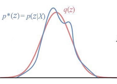 not.

  

• Then, find the setting of the parameters that makes the choosen distribution close to the posterior of interest.

• One method to achieve the variational inference is KL divergence

Kullback-Leibler (KL) Divergence

• KL divergence measures the closeness of two distributions.

  Higher the probablity of an event, lower will be its information content. i.e information is inversly proportional to the probability of the event.
  For example : Lower temperature at any day on june(summer) is less likely but it has high information content about the weather conditions of that day.

• Information Content of an event $X$ w.r.t some probabilty distribution $\{p,q\}$.

  $I_p(x) = -log(p(x)) \newline I_q(x) = -log(q(x))$

• KL divergence is the Expectation value of the change in information content

  $D_{KL}(q(x)||p(x)) = E_{\sim{q}}{[\Delta{I}]} = \int{q(x)log\biggl(\frac{q(x)}{p(x)}\biggr)}dx$

• Kullback-Leibler (KL) is not symmetric.

  $DL(q(x)||p(x)) \neq DL(p(x)||q(x))$

• Evidence Lower Bound (ELBO) :

  • We actually can’t minimize the KL divergence exactly, but we can minimize a function that is equal to it up to a constant.

What VAE Offers

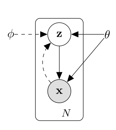
• As naive bayes says that computation of $p(z)p(x|z)$ is a generative modelling problems so, starting from that,

• Assume $p_{\theta}(z)p_{\theta}(x|z)$ as generative model, but for the computation of the equation there is a requirement of posterior $p_{\theta}(z|x)$ which is forms the equation.

  $p_{\theta}(z|x) = \frac{p_{\theta}(z)p_{\theta}(x|z)}{p_{\theta}(x)} \tag{1}$

• Due to $p_{\theta}(z|x) = \int_z{p(x|z)p(z)dz}$ which is intractable whole equation 1 become intractable.

• So using variational inference, assume a variational Approximation $q_{\phi}(z|x)$ (Which works as a recognition model) for the $p_{\theta}(z|x)$.

• Now there are method to find the parameters $\phi$ for $q_{\phi}(z|x)$ called Variational Bayesian methods, like mean-field Variational inference, Factorized approximation, KL divergence.

• But in VAE parameters $\phi$ for $q_{\phi}(z|x)$ are learned jointly with the generative model parameters $\theta$.

VAE Loss function Derivation

$L(\phi, \theta) = - E_{\sim{q}}log(p(x|Z)) + D_{KL}(q_{\phi}(Z|x) || p_{\theta}(Z))$

$\begin{aligned} D_{KL}(q_{\phi}(Z|x) || p_{\theta}(Z|x)) &= E_{q_{\phi}(Z|x)}(I_p -I_q) \\ &= E_{q_{\phi}(Z|x)}[log(q_{\phi}(Z|x)) - log(p_{\theta}(Z|x))] \\ &= E_{q_{\phi}(Z|x)}\biggl[log(q_{\phi}(Z|x)) - log\biggl(\frac{p_{\theta}(x|Z)p_{\theta}(z)}{p_{\theta}(x)}\biggr)\biggr] \\ &= E_{q_{\phi}(Z|x)}[log(q_{\phi}(Z|x)) - log(p_{\theta}(x|Z)) - log(p_{\theta}(Z)) + log(p_{\theta}(x))] \\ D_{KL}(q_{\phi}(Z|x) || p_{\theta}(Z|x)) - log(p_{\theta}(x)) &= E_{q_{\phi}(Z|x)}[log(q_{\phi}(Z|x)) - log(p_{\theta}(x|Z)) - log(p_{\theta}(Z))] \\ &= - E_{q_{\phi}(Z|x)}log(p_{\theta}(x|Z)) + E_{q_{\phi}(Z|x)}[log(q_{\phi}(Z|x)) - log(p_{\theta}(Z))] \\ &= - E_{q_{\phi}(Z|x)}log(p_{\theta}(x|Z)) +D_{KL}(q_{\phi}(Z|x) || p_{\theta}(Z)) \\ log(p_{\theta}(x)) - D_{KL}(q_{\phi}(Z|x) || p_{\theta}(Z|x)) &= E_{q_{\phi}(Z|x)}log(p_{\theta}(x|Z)) - D_{KL}(q_{\phi}(Z|x) || p_{\theta}(Z)) \end{aligned}$

NOW : $D_{KL}(q_{\phi}(Z|x) || p_{\theta}(Z|x)) \geq 0$
Proof : //TODO

• On combining above two equations

$log(p_{\theta}(x)) \geq E_{q_{\phi}(Z|x)}log(p_{\theta}(x|Z)) - D_{KL}(q_{\phi}(Z|x) || p_{\theta}(Z))$

• The right hand side of the equation is the Evidence Lower Bound (ELBO) :
• Therefore maximizing the ELBO maximizes the log probability of our data by proxy. This is the core idea of variational inference
• Kullback-Leibler term in the ELBO is a regularizer because it is a constraint on the form of the approximate posterior.
• second term is called a reconstruction term because it is a measure of the likelihood of the reconstructed data output at the decoder.
• Negation of the ELBO is the loss function for VAE

Derivative of loss function

• For wait upgradation there is need of $\nabla{L(\phi, \theta)}$ which is $\nabla_{\phi}{L(\phi, \theta)}$ taking $\theta$ as constant and $\nabla_{\theta}{L(\phi, \theta)}$ taking $\phi$ as constant

• Derivation w.r.t $\theta$ is OK but w.r.t $\phi$ is problematic because of the $E_{q_{\phi}(Z|x)}log(p_{\theta}(x|Z))$ as the Expectation depends on the variable $\phi$

• Using Monte Carlo estimation

$log(p_{\theta}(x)) \geq \frac{1}{L}\sum_{i=1}^{L}{log(p_{\theta}(x|Z))} - D_{KL}(q_{\phi}(Z|x) || p_{\theta}(Z))$

• Reparameterization Trick

• This strategy is used to make monte carlo estimate of Expectation differentiable by rewriting the Expectation with respect to $q_{\phi}(Z|x)$

Matrix Maths and Training

Conditional Variational Autoencoders

Adversarial Autoencoders

Tensorflow Implementation

Full Implementation of different Autoencoder is Available on my kaggle account link is here

References

1. Chapter 14: Autoencoders {Deep Learning; Ian Goodfellow}.

Comments